Algorithmic differentiation and gradient descent in JavaScript

(This is the fourth article in the series for Golf Horse: Wordle.)

In our previous article about building a model for probabilities of English letters, we had a number of parameters to optimize. In this article, we’ll go through some numerical techniques to find optimal values of a function. Note that this optimization code is not part of the Golf Horse submission. Rather, it was used to find parameters I included in the submission.

There are two main ideas we’ll cover: algorithmic differentiation (AD for short), and gradient descent (GD for short). AD is a cool technique to get derivatives of any function, and GD is a method for using derivatives to find the minimum of a function. Both these techniques are used extensively in machine learning as well as other large optimization problems. We’ll illustrate them with JavaScript code—not because JavaScript is good for numerical code, but because that’s what I used myself when working on the Golf Horse submission.

The code accompanying this post is available on GitHub.

Algorithmic differentiation

Given a program with numerical inputs and outputs, AD is a technique to transform the program so that it also outputs its derivatives. AD comes in two main variants: “forward” AD will calculate the derivatives of all the outputs with respect to one input, and “reverse” AD will calculate the derivatives of one output with respect to all the inputs. Reverse AD is also known as adjoint AD and, when used in neural networks, backpropagation. In the context of optimization problems, we usually only have one output (e.g., some objective function), so reverse AD is the more common technique.

The cool thing about AD is that it only requires a small constant factor overhead, around 5-10x in my experience. If you haven’t seen AD before, I’d like you to take a moment to be amazed. If some wildly complex function has a million inputs, I can get all million partial derivatives with only a 10x increase in computation! This opens up a lot of opportunities for efficient numerical algorithms, including GD, which we’ll look at later in this article.

We’ll focus exclusively on reverse AD here, as that’s what we’ll need for GD.

The mathematical idea behind AD is to repeatedly apply the chain rule from calculus—and frankly, that’s really all there is to it. (If you’d like the details, Wikipedia has them.) For reverse AD, it’s a little tricky because we have to essentially run the program backwards to apply the chain rule appropriately. In order to run the calculations backwards, we’ll store them all in a graph. Let’s begin by setting up the data structures for the calculation graph. Each node will look like this:

example_aad_node = { 
  value: 1.23, //numerical result of this node
  parents: [], //all the input nodes
  ddparents: [] //derivative of this node wrt each of the parents
}

Because we’ll need the calculation graph to be topologically sorted (i.e., an order such that the parents of a node precede it), it saves a lot of trouble if we store it in a stack. To initialize the stack,

function aad_begin()
{
  aad_stack = [];
}

(This creates a mutable global variable, which I rather dislike in production code, but this isn’t production!) To create a node for a constant number,

function aad_const(c)
{
  var node = {
    value: c,
    parents: [],     //no inputs to a constant!
    ddparents: []
  };
  aad_stack.push(node);
  return node;
}

Mathematical operations are more interesting because the parents and derivatives are non-trivial:

function aad_add(node1, node2)
{
  var ret = {
    value: node1.value + node2.value, 
    parents: [node1, node2], //inputs to our addition
    ddparents: [1, 1] //derivative is 1 for addition
  };
  aad_stack.push(ret);
  return ret;
}

function aad_mul(node1, node2)
{
  var ret = {
    value: node1.value * node2.value, 
    parents: [node1, node2], //inputs to our multiplication
    //d/dx(xy) = y, d/dy(xy) = x
    ddparents: [node2.value, node1.value]
  };
  aad_stack.push(ret);
  return ret;
}

function aad_log(node)
{
  var x = Math.log(node.value);

  //Catch errors to help debugging
  if(isNaN(x))
    throw "NAN from log(" + node.value + ")";

  var ret = { 
    value: x, 
    parents: [node], 
    //d/dx(log(x)) = 1/x
    ddparents: [1 / node.value]
  };
  aad_stack.push(ret);
  return ret;
}

(Obviously there are lots more operations we could support, see the GitHub code for more.)

Finally, we have the crux of reverse AD, where we calculate all the derivatives. We start with the last node and walk up the calculation graph, accumulating all the partial derivatives. We’re going to store the partial derivatives in the nodes themselves. Here’s the function:

function aad_calc_derivs()
{
  //Start with the final node. Derivative of the node wrt itself is 1
  aad_stack[aad_stack.length - 1].derivative = 1;

  //Walk up the calculation graph
  for(var n = aad_stack.length - 1; n >= 0; n--)
  {
    var node = aad_stack[n];

    //Apply chain rule to each parent of the node
    for(var i = 0; i < node.parents.length; i++)
    {
      var parent = node.parents[i];
      parent.derivative = (parent.derivative || 0) + 
        node.ddparents[i] * node.derivative;
    }
  }
}

After calling aad_calc_derivs, every node is now populated with its partial derivative in the field derivative.

Here’s an example of our AD code in action. Let’s say we want to get the gradient of \(\log(x_1y_1+x_2y_2 + x_3y_3 + x_4y_4)\) where \(x=[1,2,3,4]\), \(y=[2,3,4,5]\):

aad_begin();
var xs = [1, 2, 3, 4].map(aad_const);
var ys = [2, 3, 4, 5].map(aad_const);
var sum = aad_const(0);
for(var i = 0; i < 4; i++)
  sum = aad_add(sum, aad_mul(xs[i], ys[i]));
var result = aad_log(sum);
aad_calc_derivs();

console.log("Value of function: " + result.value);
console.log("Derivatives wrt xs: " + xs.map(x => x.derivative));
console.log("Derivatives wrt ys: " + ys.map(y => y.derivative));

/*
Output is:
Value of function: 3.6888794541139363
Derivatives wrt xs: 0.05,0.07500000000000001,0.1,0.125
Derivatives wrt ys: 0.025,0.05,0.07500000000000001,0.1
*/

Pretty slick, right? (Though the lack of operator overloading in JavaScript makes numerical code annoying…)

Now that we can get gradients for cheap, let’s look at how they can be used for optimization.

Gradient Descent

Suppose we have a function f that we want to minimize. The idea behind gradient descent is that we start with some guess x, then move our guess in the direction where f is most rapidly decreasing. As we know from vector calculus, the direction of most rapid descent is the negative of the gradient, \(\nabla f(x)\). Therefore, we can write our iteration as

\(\displaystyle x_{i+1} = x_i – \gamma \frac{\nabla f(x_i)}{||\nabla f(x_i)||}\)

where \(\gamma\) is some constant controlling the length of the step, commonly called the “learning rate”. The learning rate requires a bit of finesse; we’ll return to it shortly.

Let’s start with a few functions for manipulating vectors in JavaScript:

function vec_scale(vec, x)
{
  return vec.map(y => x * y);
}

function vec_add(vec1, vec2)
{
  if(vec1.length != vec2.length)
    throw "unequal vector sizes";
  return vec1.map((x,i) => x + vec2[i]);
}

function vec_norm(vec)
{
  var t = 0;
  for(var i = 0; i < vec.length; i++)
    t += vec[i] * vec[i];
  return Math.sqrt(t);
}

function vec_equal(vec1, vec2)
{
  if(vec1.length != vec2.length)
    return false;
  for(var i = 0; i < vec1.length; i++)
    if(vec1[i] != vec2[i])
      return false;
  return true;
}

Suppose we have a function f that returns both its value and its gradient. The stepping procedure for gradient descent will look like this:

var [y, dy] = f(x);
var direction = vec_scale(dy, -1); 
var norm = vec_norm(direction);
var new_x = vec_add(x, vec_scale(direction, step / norm));

We haven’t defined step yet; that will be the learning rate. We’ll start with a step size of 1 and adjust it up or down as we go. To prevent our step size from staying too small, we’ll scale it up after every iteration: step *= 1.1. To keep our step size from getting too big, we’ll use the Armijo rule:

\(\displaystyle f(x_{i+1}) \leq f(x_i) – c\gamma||\nabla f(x_i)||\)

where c is some constant less than 1. This rule says that after we take a step, the function has indeed decreased as predicted by the gradient. Basically, it’s ensuring we’re making a sufficient amount of progress with each step of the algorithm. (In practice, a very small value of c works best, even though it makes it look like the rule isn’t doing much.) If we fail the Armijo rule, we’ll halve the step size and try again: step *= .5.

Putting it all together, our basic gradient descent function looks like this:

function gradient_descent_minimize(f, guess, max_iter)
{
  var iter = 0;
  var step = 1;
  var x = guess;
  
  while(true)
  {
    var [y, dy] = f(x);
    var direction = vec_scale(dy, -1);
    var norm = vec_norm(direction);
    
    //Check termination condition
    iter++;
    if(step * norm <= 1e-15 * Math.abs(y) || iter >= max_iter)
      return x;
		
    //Shrink step size until we satisfy Armijo rule
    while(true)
    {
      var new_x = vec_add(x, vec_scale(direction, step / norm));
      var new_y = f(new_x)[0];
      if(y - new_y > .1 * step * norm || vec_equal(x, new_x))
        break;
      step *= .5;
    }
    
    //Update for next iteration
    step *= 1.1;
    x = new_x;
  }
}

The gradients we get from AD combine with GD to form a powerful framework for optimization. Here’s an example of using GD to optimize a nontrivial function:

/*
We optimize the y_i such that the total length of the path:
  (0,0),
  (.01, y_1),
  (.02, y_2),
  ...
  (.99, y_99),
  (1,1)
is minimized.
*/

function objective_function(heights)
{
  //Set up AAD
  aad_begin();
  heights_aad = heights.map(aad_const);

  //Sum up distances of 100 segments
  var total_length = aad_const(0);
  for(var i = 0; i < 100; i++)
  {
    var left_height  = i == 0  ? aad_const(0) : heights_aad[i-1];
    var right_height = i == 99 ? aad_const(1) : heights_aad[i];
    var height_diff = aad_sub(left_height, right_height);
    var length = aad_pow(
      aad_add(aad_const(.0001), aad_mul(height_diff, height_diff)),
      aad_const(.5));
    total_length = aad_add(total_length, length);
  }
	
  //Run AAD
  aad_calc_derivs();

  //Return the total error and the gradient
  return [total_length.value, heights_aad.map(c => c.derivative)];
}

var result = gradient_descent_minimize(
  objective_function, 
  Array(99).fill(0),
  10000);

Running this program gives a solution of length 1.4174, compared to the optimal solution of \(\sqrt{2}=1.4142\).

This problem is poorly suited to gradient descent, so it requires a lot of iterations before it starts to converge. But it illustrates that AD and GD can scale to optimizations with many parameters.

Though useful for a lot of problems, GD has a pretty significant limitation: its convergence rate is only \(O(1/n)\). Though out-of-scope for this article, I want to mention that there are various enhancements to GD to help improve speed and convergence, and other algorithms such as BFGS which have a better theoretical convergence rate.

Optimizing my submission

Having a decent AD/GD framework in place was invaluable for allowing me to experiment with different models and approaches. I could leave dozens or even hundreds of free parameters, run the optimization, and quickly get results. Even with my basic GD implementation, a few minutes of computation would usually converge enough to give a sense whether I was headed in the right direction.

In the previous article, I described the models my submission used. The free parameters are:

• The initial counts used for context models. This comprises two parameters: the initial “true” count and “false” count. (All context models used the same initial counts. I experimented with different initial counts, but it wasn’t very helpful.)
• For each context model, the coefficient and exponent used in the mixing formula. There are 6 context models, so 12 parameters.

(Note: The decay coefficient for counts is another free parameter, but I hand-optimized it rather than using AD/GD due to my specific implementation limitations.)

In total, that’s 14 parameters, which is actually quite a small number. Indeed, every additional parameter takes additional code space, so I was always trying to minimize the free parameters in the final model.

However, though the parameter dimension was small, the function we’re minimizing is complex. We are evaluating our model on 306384 bit predictions, which typically used several seconds of CPU time. So, our function evaluation was quite expensive, making each iteration of GD slow. During experimentation, I would sometimes use stochastic gradient descent to speed up the optimization: instead of evaluating the models on all 306384 bits, I would use a random subset of the bits (10% or even 1%) to get an approximate gradient. There are multitudes of additional techniques that could be used for even more speed ups, but I didn’t feel they were necessary for my workflow. If I ever attack one of the bigger Golf Horse problems, I would definitely try SAGA and BFGS.

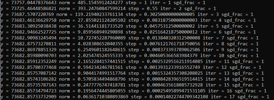
For the final submission, I let my computer run overnight to get fully optimized parameters. Then, I manually rounded off the parameters to minimize the sum of the code size (which gets smaller with less parameter digits) and the compressed data size (which gets larger as the parameters are farther away from their optimal values). In the end, somewhat surprisingly, I only needed 1-2 significant digits for the parameters, so very little code size was needed to store the parameters.

I’m afraid I won’t be sharing my final parameters—that would make it a bit too easy for others to defeat my submission!—but I hope this article provided a good enough summary of how it was done.