Modeling 5-letter English words

(This is the third article in the series for Golf Horse: Wordle.)

For our JavaScript code golf challenge, we’re compressing a list of 12947 5-letter words—the source dictionary used by the popular game Wordle.

A critical component of data compression is being able to predict data. The better you can predict, the better you can compress. In this case, that means we’re trying to predict letters that form valid English words.

I believe that the prediction model is the most important aspect of this code golf challenge. The savings I gained from improving my prediction models far outweighed the savings I gained from anything else. This is also one of the most open-ended parts of the challenge, because it involves trying to capture the rules of English orthography in as little code as possible.

In this article, we’ll cover a few related topics:

• A brief introduction to the mathematics
• How my submission represents the word list
• What is context modeling, and what context models my submission used
• What is context mixing, and what context mixing my submission used

Mathematics of compression

I’d like to give a light introduction to the mathematical relationship between prediction and data compression. This section isn’t strictly necessary to understand the rest of the article, but I believe it’s conceptually extremely useful.

To make this presentation as concrete as possible, I’m going to derive the math based on the arithmetic coder we discussed in the previous article. (This is actually backwards—of course the theory came first, and the arithmetic coder is based on the theory!) To recap, the arithmetic coder works as follows:

• Let \(p_i\) be the probability of the ith bit being 0. Let \(b_i\) be the value of the ith bit.
• Start with the interval [0,1).
• Recursively split the interval proportionally into \((p_i):(1-p_i)\), choose the first interval if \(b_i=0\) and the second if \(b_i=1\). Do this for all i.
• Choose a real number r in the final interval with finite base-b representation.
• This base-b representation of r is the compressed data.

We’re trying to optimize the amount of compressed data we output, which means we’re trying to minimize the length of the base-b representation of r. Since r must be specified accurately enough to land in the final interval, we generally need more digits the smaller the final interval is.

Let’s introduce some more notation: let n be the number of bits we’re encoding. Let \([x_i, y_i)\) be the ith interval created by the algorithm, so that \((x_0, y_0) = (0, 1)\) and \([x_n, y_n)\) is the final interval.

We have the constraint that \(r \in [x_n, y_n)\). The typical number of base-b digits d we need to specify such an r is \(-\log_b (y_n – x_n)\). Fewer digits than that is insufficient to ensure we have a value in the interval.

So, our goal should be to optimize for the log of the interval length. Observe that the interval length follows these rules:

• \(y_0-x_0=1\), because we start with the interval [0,1)
• If \(b_i=0\), then \(y_{i+1} – x_{i+1} = p_i(y_i-x_i)\).
• If \(b_i=1\), then \(y_{i+1} – x_{i+1} = (1-p_i)(y_i-x_i)\).

Let \(q_i\) be the objective probability that bit i is 0 (whereas \(p_i\) is our guess for the probability, not the true objective probability). Then we can write an equation for the expected log interval length by summing the two cases \(b_i=0\) and \(b_i=1\):

\(\displaystyle \mathbb{E}[\log(y_{i+1}-x_{i+1})] = q_i\log(p_i(y_i-x_i)) + (1-q_i)\log((1-p_i)(y_i-x_i))\)

\(\displaystyle = q_i(\log(p_i) + \log(y_i-x_i)) + (1-q_i)(\log(1-p_i) + \log(y_i-x_i))\)

\(\displaystyle = \log(y_i-x_i) + q_i\log p_i + (1-q_i)\log(1-p_i)\)

If we define \(H_i = -\log(y_i-x_i)\) (I chose the notation \(H_i\) because it’s essentially the information entropy, which is denoted by H), we can write it succinctly as:

\(\displaystyle \mathbb{E}[H_{i+1}] = H_i – q_i\log p_i – (1-q_i)\log(1-p_i)\)

To minimize \(H_{i+1}\), it’s clear that’s equivalent to maximizing \(q_i\log p_i + (1-q_i)\log(1-p_i)\). The \(q_i\) are fixed, so \(p_i\) is the parameter we optimize. The most straightforward way to optimize is to take a derivative and set to zero:

\(\displaystyle 0 = \frac{d}{dp_i} q_i\log p_i + (1-q_i)\log(1-p_i)\)

\(\displaystyle 0 = \frac{q_i}{p_i} – \frac{1-q_i}{1-p_i}\)

\(\displaystyle \frac{1-q_i}{1-p_i} = \frac{q_i}{p_i}\)

\(\displaystyle (1-q_i)p_i = q_i(1-p_i)\)

\(\displaystyle p_i-p_iq_i = q_i-p_iq_i\)

\(\displaystyle p_i=q_i\)

It’s easy to verify this is a maximum by looking at the second derivative.

Therefore, we get our best data compression when the guesses for probabilities \(p_i\) match the objective probabilities \(q_i\).

Representing the word list

In this section, we’ll show how we can represent the word list as a sequence of bits, which we can then use in our encoder/decoder.

The word list begins as follows:

aahed
aalii
aargh
aarti
abaca
abaci
aback
abacs
abaft
abaka

Perhaps the most obvious representation would be as a string:

"aahed aalii aargh aarti abaca abaci aback abacs abaft abaka"

However, this representation doesn’t reflect the underlying structure of the data: the words are all unique, but a string can contain duplicate words. Instead, a prefix tree naturally represents the uniqueness of each word:

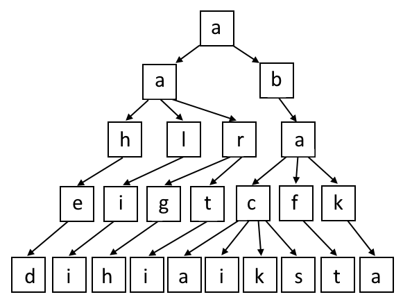
Technically, we’ll actually have 26 prefix trees, one for each possible first letter.

With this setup, each path from a root to a leaf represents a word from our word list. Note that all such paths have length 5, since all our words are 5 letters.

To store this prefix tree, for each internal node, we’ll have 26 bits to record which letters are children. For example, the root “a” will have its first two bits true, because “a” and “b” are children, and the remaining 24 bits false. The “a” in the second row will have the bits for “h”, “l”, and “r” true, and the rest of the bits false.

In my submission, I simply go through the nodes in depth-first order alphabetically and decode the bits for each node as we visit them. We end up with 306384 bits for the full word list.

I was happy about this representation:

• It is represented with bits, so I didn’t need to create a range decoder.
• It naturally enforces the uniqueness of each word.
• As we build the trees, we have a lot of context available to use for predicting each bit. For example, we have the parents (i.e., previous letters of the word) as well sibling nodes’ (i.e., words that share a prefix) information. Which naturally segues into the next section about context modeling!

Context modeling

Context modeling is just what it sounds like: when predicting a bit, we look at the context (i.e., surrounding environment of previous bits) and apply a model to guess the next bit (or more precisely, the probability of the next bit being true). The idea is to use a bunch of context models to make reasonable guesses for the next bit; later we’ll see how to combine these guesses.

The simplest context is nothing. This means we’d be making blind predictions for the next bit. Although not very useful in real problems, it’s not worthless either. For example, if we know 20% of the bits are true, a blind context model can still use that information.

The next simplest example of a context is what letter we’re predicting. Though this context model is minimal, it’s still useful, because even without any other information, we know a letter like “e” is much more likely to be valid than “z”.

A more interesting context model is the letter we’re predicting plus the preceding letter. This context model allows us to express facts such as “h” being likely to follow a “t”, but not an “f”.

For each context, we keep a count of how many times the bit was true or false. For example, every time an “e” is valid, we’d add to the count for “e:true” (“e” being the letter and “true” being the bit), and if it’s not valid, we add to the count for “e:false”. For another example, suppose “h” is preceded by “t”. If it’s valid, we’d add to the count for “th:true”, else we add to the count for “th:false”.

There’s a nuance to mention: it’s inconvenient to start counting at 0 because it creates division-by-0 problems when we try to infer a probability from the counts. In practice, we initialize the counts to some predefined constants. For example, we might set all the “true” counts to 0.1 and all the “false” counts to 0.4; then the implied probability starts at 0.1/(0.1+0.4) = 20%. In my submission, these starting values were parameters that I optimized—I’ll explain the optimization in the next article.

Furthermore, there’s a trick that often helps make context counts more useful, and that’s to apply some decay to the counts. For example, each time we do a prediction for “e”, we’d first multiply the counts “e:true” and “e:false” by 95%. This trick will reduce the weight of older data, with the hope that newer data is more relevant. Indeed, I found a small amount of decay improved the results of my program.

Contexts that worked well

I spent a lot of time experimenting with context models, trying out as many ideas as I could come up with. Here are the high-level ideas that really paid off:

• Contexts for previous letters. Nothing fancy here, these are standard contexts used for modeling text.
• Vowel-consonant patterns for previous letters. Based on my testing, it’s best that “Y” counts as a vowel, “W” doesn’t.
  This context is effective because English tends to limit the number of vowels and consonants that can occur consecutively. It’s rare to have 3 vowels in a row, for example. If we see “ee”, “ei”, or “oo”, we should bet that the next letter is a consonant.
  Although the contexts for previous letters will also effectively capture vowel-consonant patterns, it takes a lot more data before these contexts get statistically useful counts. There are 26 * 26 = 676 2-letter contexts, but only four 2-letter vowel-consonant patterns.
• The current letter position, i.e., whether it’s the second, third, fourth, or fifth. There are a couple reasons this is really important:
  • Earlier positions tend to have more children, and thus a higher probability of their bits being true. The explanation is simply that the shorter the prefix, the more possible words start with that prefix.
  • “S” frequently occurs in the last position, because it’s used to pluralize words. Similarly, there are other common suffixes that cause statistics to look different in the last positions compared to earlier positions.
• Recall that for each node, we record 26 bits representing which letters are children of the node. As we produce these bits, we can track how many are true. It turns out this is very useful as a context, although it’s less obvious why.
  • With how we construct the tree, we are guaranteed that at least one bit will be true, i.e., the node has at least one child. If we get through 25 bits and none are true, we know the 26th better be true!
  • There are some correlations between valid children, and tracking the number of true bits helps model these correlations. I suspect there’s a lot of interesting behavior here, but I didn’t investigate enough—this is a potential area of improvement in my future attempts!

In the end, I used six context models for my submission:

1. The combination of the position, the letter being considered, and the number of true bits seen so far for this node
2. #1 plus the preceding letter (except positions two and three are grouped together; otherwise there’s not enough data for position two)
3. #2 plus the next preceding letter (i.e., 2 previous letters)
4. The combination of the position, the letter being considered, and the previous 3 letters
5. The combination of the position, the letter being considered, the preceding letter, and the vowel/consonant classification of the next preceding letter
6. #5 plus the vowel/consonant classification of the next preceding letter

Note that #3 and #5 apply only for letters in the third or later position, and #4 and #6 only for the fourth or fifth position.

You may notice some inconsistencies in the context models: some include the count of true bits seen, some don’t; #5 and #6 look at letters in some positions and vowel/consonant classification in other positions. This is simply because in my testing, these combinations performed best.

Context mixing

Context mixing is the method used to combine the data from the context models and produce a probability that the next bit is true.

To take a motivating example, let’s suppose we’re considering the letter “b” and the previous letter was “s”. Our context model for “b” alone says that of 100 occurrences, 8 were true and 92 were false, suggesting an 8% probability. Our context model for “b” preceded by “s” says that of 10 occurrences, 0 were true and 10 were false, suggesting a 0% probability. How should one combine the estimates of these models? On the one hand, the model for “b” preceded by “s” is more specific—it considers the previous letter—so we should trust it more. On the other hand, there are only 10 samples for it, compared to 100 samples for the other context model, so it has a larger statistical error. (If you’re curious, there are two words that do have the pattern “sb”: “busby” and “isbas”.)

Unfortunately, there is no principled mathematical approach to combining context models. Instead, we must rely on heuristics and empirical tests.

A typical approach used in data compression algorithms is to apply some learning algorithm that adjusts weights for each model, increasing the weight on models that have been producing better estimates. While this approach certainly can work, the convergence is slow. In my testing, I couldn’t get adaptive weights to outperform optimized static weights. (I still wonder if I had a bug, I expected adaptive weights to do better.)

I figured that I should be able to come up with a formula that works better than static weights. I wanted the formula to take into account which context models were more specific (e.g. #2 is more specific than #1) and put more weight on them, but I also wanted to take into account the statistical significance of each context model (models with low counts aren’t reliable).

My idea was to weight each model by a formula of the form \(a(count)^b\), where a and b are constants that I’ll optimize. (I’ll discuss optimization in the next article.) More specific models can have a larger b, which will cause their weight to dominate as their count increases. Less specific models can have a small b so that their weight stays small. In fact, context model #1 has b=0.

To give the specifics, our context mixing formula is

\(\displaystyle \sigma\left(\frac{\displaystyle \sum_{i=1}^6 a_i(c_i)^{b_i}\sigma^{-1}(r_i)}{\displaystyle \sum_{i=1}^6 a_i(c_i)^{b_i}}\right)\)

where \(\sigma\) is the logistic function, \(a_i, b_i\) are constants, \(c_i\) is the count for the ith context model, and \(r_i\) is the probability implied by the ith context model (that is, the count for “true” divided by the total count).

(Why do we use the logits rather than simply averaging together the \(r_i\)? It performs better! I don’t know if there’s any deeper reason, but logits are widely used in machine learning and data compression precisely because they tend to perform better.)

Actually, I had a fortuitous bug in my program that improved on this formula. The numbers \(c_4, c_5, c_6\) were all set equal to \(c_3\) due to a copy-paste mistake. When I fixed the bug, my compression ratio got worse! Naturally, I left the bug in there, and tried experimenting with similar “bugs”, but couldn’t find anything better. So our final formula becomes

\(\displaystyle \sigma\left(\frac{\displaystyle \sum_{i=1}^6 a_i(c_{\min(3,i)})^{b_i}\sigma^{-1}(r_i)}{\displaystyle \sum_{i=1}^6 a_i(c_{\min(3,i)})^{b_i}}\right)\)

Why would this bug improve on the formula? At first, it seemed unprincipled to me; why shouldn’t the weight for model #4 be based on the counts for model #4? I don’t have a complete answer. My best theory is that there’s some strange phenomenon where sometimes low-count models are preferred. For example, let’s say that context #3 has a high count, but context #4 has an unusually low count. If we weighted them according to counts, then #3 would get the higher weight. However, the fact that #4 has been so rare suggests maybe we’re in an exceptional case where #3 isn’t reliable. So, we shouldn’t be weighting #3 so highly. By unifying the counts for models #3-6, we prevent this situation from occurring. In any case, this mystery suggests there’s still lots of room to innovate with context mixing.

Compression results

First, let’s do some math to see how we can calculate the amount of data needed for arithmetic encoding. Observe:

• The number of bits needed for the arithmetic encoding is \(-\log_2 (y_n – x_n)\), where \(y_n-x_n\) is the length of the final interval.
• If \(b_i=1\) (that’s the ith bit), then \(y_{i+1} – x_{i+1} = p_i(y_i-x_i)\), where \(p_i\) is the probability coming from our model.
  If \(b_i=0\), then \(y_{i+1} – x_{i+1} = (1-p_i)(y_i-x_i)\).

Thus, we can calculate the encoded size as

\(\displaystyle -\sum_{i=0}^{n-1} \log_2\left\{\begin{array}{lr}p_i & \text{if } b_i=1\\ 1-p_i & \text{if } b_i=0\end{array}\right.\)

We started with 306384 bits needed to describe the prefix tree. With our models and optimized parameters, we only need 73663 bits for the arithmetic encoder. That gives a compression ratio of 4.16.